library(igraph)
library(ADAPTSNA)15 Dynamic Network Visualisations
| LEARNING ELEMENTS - Data Practices |
|---|
|
You might be interested in networks that change over time. Rather than a cross-section of relationships, you may have multiple networks that are taken at different time points. These are called discrete longitudinal networks. They are discrete because each network represents a discrete, distinct, point in time. For example, you may have monthly phone call data between people and their family. You may have yearly romantic affiliations between a group of people. The point is, the time stamps are distinct and standardised (yearly, monthly, daily etc.) and the relationships may change over time. There is such a thing as continuous longitudinal network data, but we will just focus on discrete networks for now.
In other tutorials we have been using collaboration data between Grime musicians. Well, we can measure this over time! This next chunk should seem familiar to you, they bring in and clean up edgelists of collaborations every two years from 2008-2014 (four time stamps).
# 2008
edge_list <- load_data("GRIME_2008_Edge.csv", header = TRUE)
grime_08<- graph_from_data_frame(d=edge_list, directed = TRUE)
##Removing Loops
grime_08 <- delete_edges(grime_08, E(grime_08)[is.loop(grime_08)])


# 2010
edge_list_10 <- load_data("GRIME_2010_Edge.csv", header = TRUE)
grime_10<- graph_from_data_frame(d=edge_list_10, directed = TRUE)
##Removing Loops
grime_10 <- delete_edges(grime_10, E(grime_10)[is.loop(grime_10)])

# 2012
edge_list_12 <- load_data("GRIME_2012_Edge.csv", header = TRUE)
grime_12<- graph_from_data_frame(d=edge_list_12, directed = TRUE)
##Removing Loops
grime_12 <- delete_edges(grime_12, E(grime_12)[is.loop(grime_12)])

# 2014
edge_list_14 <- load_data("GRIME_2014_Edge.csv", header = TRUE)
grime_14<- graph_from_data_frame(d=edge_list_14, directed = TRUE)
##Removing Loops
grime_14 <- delete_edges(grime_14, E(grime_14)[is.loop(grime_14)])
Now we have the networks in, we need to switch gears a little over to another package that allows us to you create an object known as a network list. Like it sounds, it is a list of networks. We use the package intergraph to swap from igraph over to an object type “Network” that the packages Networkdynamic and ndtv recognise as they are the ones we will use for our visualisaitons. We also detach igraph since we are no longer using that package. We want to detach it so R does not get confused if there are functions that are similarly worded across packages.
library(intergraph)
grime_net_1 <- asNetwork(grime_08)
grime_net_2 <- asNetwork(grime_10)
grime_net_3 <- asNetwork(grime_12)
grime_net_4 <- asNetwork(grime_14)
If you take a look at these networks, the appear a little different from our usual igraph object but have the same information stored.
grime_net_1 Network attributes:
vertices = 40
directed = TRUE
hyper = FALSE
loops = FALSE
multiple = FALSE
bipartite = FALSE
total edges= 28
missing edges= 0
non-missing edges= 28
Vertex attribute names:
vertex.names
Edge attribute names:
collab_weight Right, now the fun stuff. We need to bring in our new packages and then create our dynamic network object using the networkdynamic() function.
detach("package:igraph", unload=TRUE)
library(networkDynamic)
library(ndtv)

net_dynamic_4periods <- networkDynamic(
  network.list = list(grime_net_1,
                      grime_net_2,
                      grime_net_3,
                      grime_net_4),
  vertex.pid = "vertex.names")
Neither start or onsets specified, assuming start=0
Onsets and termini not specified, assuming each network in network.list should have a discrete spell of length 1
Argument base.net not specified, using first element of network.list instead
Initialized network of size 91 inferred from number of unique vertex.pids
Created net.obs.period to describe network
Network observation period info:
Number of observation spells: 1
Maximal time range observed: 0 until 4
Temporal mode: discrete
Time unit: step
Suggested time increment: 1 Note that you have to state the vertex.names as the id. There are artists in these networks that come and go (known as joiners or leavers). setting the vertex.pid ensures that R recognises all artists based on these unique identifiers.
Let’s take a look at this new dynamic network object.
net_dynamic_4periodsNetworkDynamic properties:
distinct change times: 5
maximal time range: 0 until 4
Includes optional net.obs.period attribute:
Network observation period info:
Number of observation spells: 1
Maximal time range observed: 0 until 4
Temporal mode: discrete
Time unit: step
Suggested time increment: 1
Network attributes:
vertices = 91
directed = TRUE
hyper = FALSE
loops = FALSE
multiple = FALSE
bipartite = FALSE
vertex.pid = vertex.names
net.obs.period: (not shown)
total edges= 188
missing edges= 0
non-missing edges= 188
Vertex attribute names:
active vertex.names
Edge attribute names:
active This object tells us all about the network over time. Pay special attention to the time range. We have four networks and this ojbect confirms that there are four time periods (0 - 4).
You can make this a data frame to observe changes in tie formation. Pay attention to the onset and terminus columns. These indicate when ties form and dissolve. Head and tail columns indicate a “to” and “from” logic.
net_dynamic_4periods_dat <- as.data.frame(net_dynamic_4periods)

head(net_dynamic_4periods_dat)
onset terminus tail head onset.censored terminus.censored duration edge.id
1 0 1 1 89 FALSE FALSE 1 1
2 0 1 69 89 FALSE FALSE 1 2
3 0 1 9 89 FALSE FALSE 1 3
4 0 1 24 89 FALSE FALSE 1 4
5 0 1 81 89 FALSE FALSE 1 5
6 0 1 26 89 FALSE FALSE 1 6Now we can start making some visualisations. First, we can create a time prism of the networks.
compute.animation(net_dynamic_4periods)slice parameters:
start:0
end:4
interval:1
aggregate.dur:1
rule:latesttimePrism(net_dynamic_4periods,at=c(0,1, 2,3),
displaylabels=FALSE,planes = TRUE,
label.cex=0.5)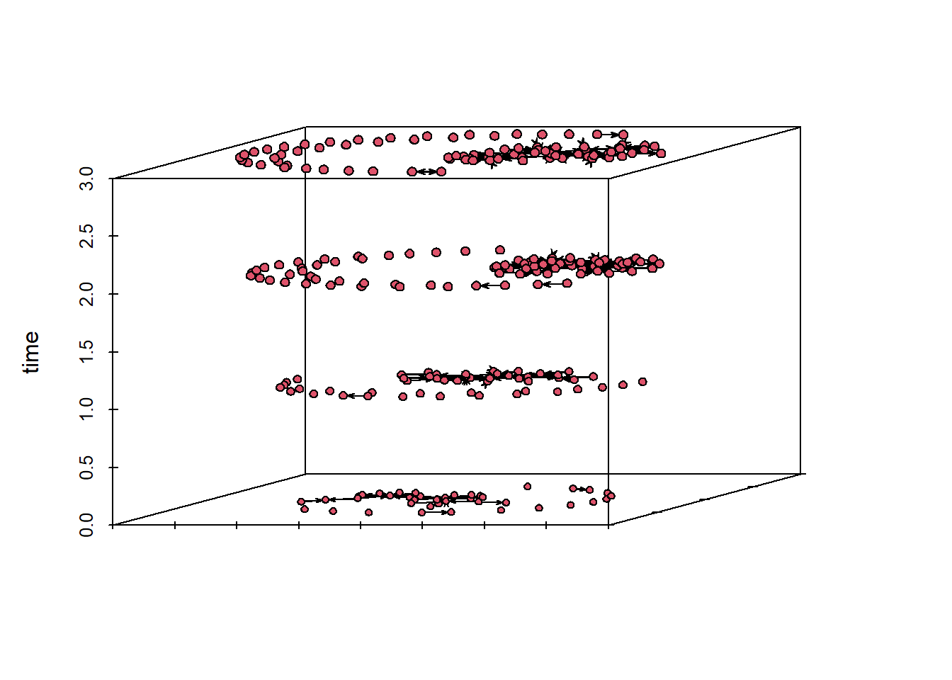
With this network object, we are ready to look at the changes over time and present a movie using the “render.d3movie()” function from ndtv. I suggest using the “output.mode = htmlWidget” option so it keeps the video in your rstudio environment. Alternatively, you could use the “launchBrowser= T” option to open up an internet page with your video. To do this, you need to specify the filename. For example, “filename= Grime-Network.html”.
render.d3movie(net_dynamic_4periods, output.mode = 'htmlWidget')The play buttons on the bottom right operate the video. You can alter the speed of the transitions between the time points by using the options menu on the top right.
You can alter the appearance of the movie in a similar way as you can change the colours and other elements of the network.
render.d3movie(net_dynamic_4periods,
               usearrows = F,
               displaylabels = F,
               bg="black", vertex.border="white",
               vertex.col =  "blue",
               edge.col = "orange",
               output.mode = 'htmlWidget')